Value at Risk for Commodity Trading, using Tableau and R

Cadran Consultancy and Cadran Analytics work hand in hand in creating value for commodity trading companies. Because of the extensive capabilities of Tableau to run complex algorithms in R (a programming language often used by data scientists), we are excited to announce our capability of Value at Risk (VaR) models by means of Tableau. By integrating this with Arantys, companies are able to make use of a reliable transactional system, while applying complex analytical models to assess their exposure. VaR for Tableau can now be implemented alongside Arantys.

What is VaR?

For companies which hold portfolios of certain assets, the VaR is a relatively simple yet effective method for measuring the downside risk of this portfolio. This blog first explains how the VaR works, after which a VaR dashboard in Tableau is shown. If you are already familiar with the concept of VaR, you might want to skip to the Tableau dashboard below.

The concept of VaR

Let’s say that you enter a contract in which you will purchase soybeans today and have to sell them in a month from now. In other words, you have a long position in soybeans. If the market price decreases during the coming 30 days, you would make a loss on this contract. Upfront, or at any moment during these 30 days, you would be interested in the likelihood of this loss and how big it could end up being. In case a big loss is likely, you could hedge against it (for example by purchasing some asset of which the price typically moves in the opposite direction of price of soybeans) or you could try to lower your position (for example by selling the contract). The VaR is a method for defining this likelihood.

For example; a 99% 1-month VaR of $50.000 would mean that we can say with 99% confidence that you will lose no more than $50.000 in the coming month. In other words, only 1 in a 100 months you will make a loss of $50.000 or more. In order to obtain this figure of 50.000, the VaR uses the historical return (meaning soybean price fluctuations) to define the volatility of soybeans. If large price drops (historically) occur often for soybeans, this will result in a higher VaR.

VaR for a portfolio of assets

This example showed just one contract for just one asset, but in reality trading companies at any moment hold many contracts in many different assets. Consider that in addition to soybeans, we also have a contract in coffee beans. Now we have a portfolio of 2 assets: soybeans and coffee beans. If we were to measure the VaR of this portfolio, we have to take into account how these two prices are correlated. In other words, what is the likelihood that both prices drop at the same time? For this, the VaR uses the covariance matrix. This matrix basically defines the relation between the different assets in the portfolio based on their historical movements.

Assorted color beans in sack

Tableau dashboard

Now that the basics of the VaR are covered, consider the Tableau dashboard below. This dashboard, which is created by combining Tableau with R, shows a VaR analysis for a portfolio with three assets. After having chosen a confidence level and a method (we will save the specifics of these methods for another blog), the dashboard shows the VaR of the portfolio. In addition, several figures are included for the individual assets:

Current exposure: the $ amount of the position
Component VaR %: the % of the portfolio VaR this asset is responsible for.
Individual VaR: the VaR of the individual asset, not considering the rest of the portfolio.

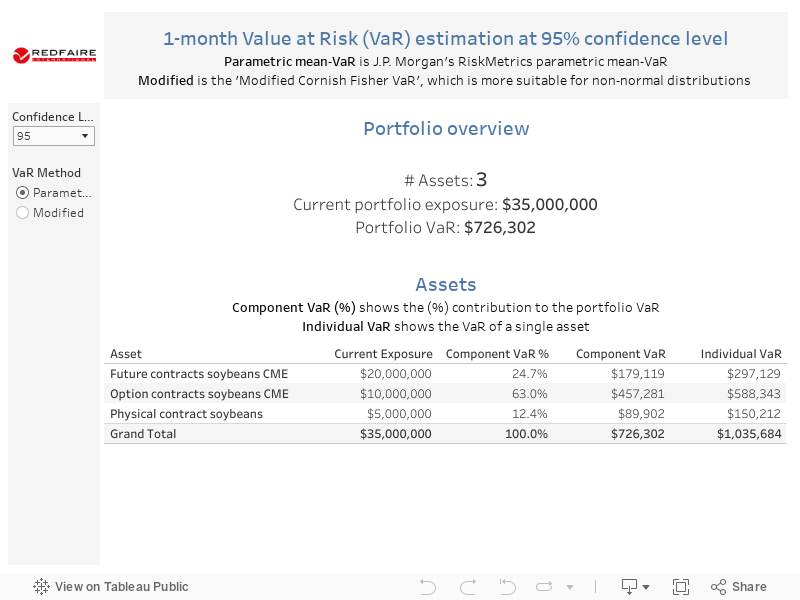
Several interesting observations can be made:

The sum of the individual VaR’s is higher than the portfolio VaR.
The reason is that by combining assets in a portfolio, this becomes diversified. Meaning that it is not likely for all three assets to significantly decrease at the same time.
The option contracts have a relatively high component VaR.
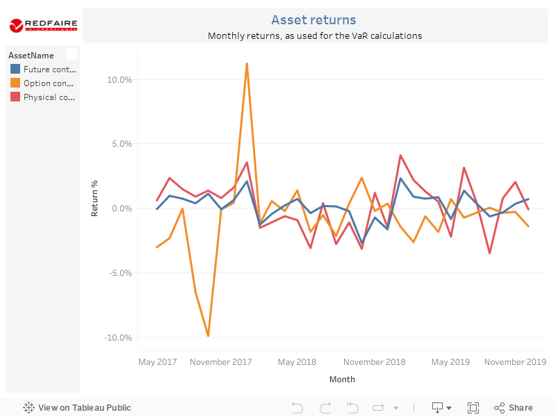
For example, with a 99% confidence level it exceeds 60% (regardless of the method chosen). So even though the exposure of the future contracts is higher, the option contracts contribute a lot more to the VaR. This is explained by the asset returns dashboard, which shows that the option contract returns are more volatile than the future contracts.
With a confidence level of 95%, the results vary greatly between the two methods.
Therefore, it is important to carefully choose a method. In case the asset returns show a non-normal distribution, the Modified method would be more appropriate than the Parametric mean-Var.

VaR with Arantys

The VaR model makes use of either historical data or market data available. Any of these models can make use of data already available in Arantys. The pre-existing data model that has been made allows Cadran Analytics to quickly unlock the potential in Tableau. Applying a more complex analytical model like VaR can be implemented at scale and with limited effort. This capability makes Tableau a scalable and future proof solution: applying new and custom models becomes easy and analyses can be made more advanced without having to deal with implementing a complex transactional layer. As also described in the blog What-If-Analytics on Trade in Tableau, and as shown in this model as well, the model can be made variable as well allowing for easy analysis by your end users.